Introduction
The chi-square test is a statistical test used for categorical data.
Example: in a survey about favorite fruits, responses fall into categories such as “apple,” “grape,” “banana,” etc.
-
Categorical example:
Favorite fruit → apple , grape, banana…
 -
Continuous example:
Height, weight → often analyzed with t-tests, ANOVA, etc.
Why Do We Need the Chi-square Test?
If we want a statistically meaningful answer, we might ask:
Is there a pattern in how people choose fruits?
For example:
Do people in their 30s like apples more than people in their 20s?
From the raw survey counts alone, it is hard to tell whether any apparent pattern is real or just random noise.
This is where the chi-square test comes in.
In simple terms, the chi-square test is a tool to check how different the observed data are from what we would expect under some assumption.
Example:
- Suppose we expect apple, banana, and grape to be equally popular (1:1:1).
- But in the actual survey, apples are far more popular than the others.
The chi-square test lets us quantify that difference and test whether it is statistically significant.
Types of Chi-square Tests
1. Goodness-of-fit Test
Checks whether the data fit a specified distribution.
Example:
- Test whether fruit preferences follow the 1:1:1 ratio for apple, banana, and grape.
2. Test of Independence
Checks whether two categorical variables are independent or associated.
Example:
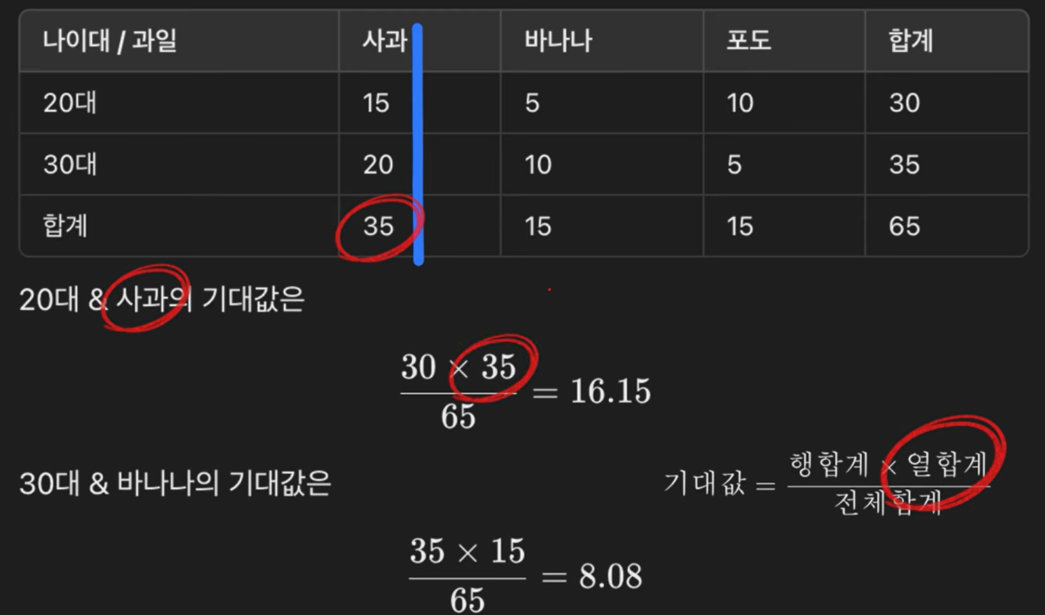
- Does “favorite fruit” depend on “age group”?
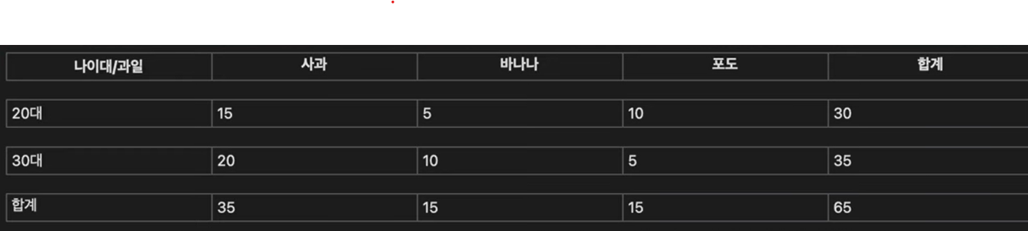
From this contingency table we can set up hypotheses.
- Null hypothesis (H_0): fruit preference does not differ by age group (fruit and age are independent).
- Alternative hypothesis (H_1): fruit preference does differ by age group (fruit and age are associated).
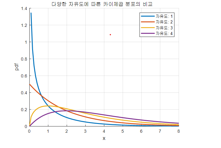
Shape of the Chi-square Distribution for Different Degrees of Freedom
By definition, the chi-square distribution is formed by summing the squares of independent standard normal random variables. Because each term is a squared value, the resulting random variable is always nonnegative, so the chi-square distribution is supported only on positive values.
Also, since it is a sum of random variables, as the number of terms being summed (the degrees of freedom) increases, the distribution becomes more symmetric and closer to a normal distribution. This behavior is a consequence of the central limit theorem.
Observed Counts vs. Expected Counts
- Observed counts: the actual counts in each cell of the table (what we see in the survey).
- Expected counts: what we would expect before seeing the data, if the null hypothesis (independence) is true.
Under the null hypothesis of independence:
- “Age” and “favorite fruit” are independent.
-
By the multiplication rule, each expected cell count can be computed as:
\[E_{ij} = \frac{(\text{row total}_i) \times (\text{column total}_j)}{\text{grand total}}.\]
Once we have all observed counts (O_{ij}) and expected counts (E_{ij}), we can compute the chi-square statistic:
\[\chi^2 = \sum_{i,j} \frac{(O_{ij} - E_{ij})^2}{E_{ij}}.\]Degrees of Freedom
For an (r \times c) contingency table:
\[\text{df} = (r - 1) \times (c - 1).\]Chi-square Distribution and Critical Values
Given the chi-square statistic (\chi^2) and the degrees of freedom (\text{df} = k), we can:
- Use software (R, Python, calculator) to find the p-value, or
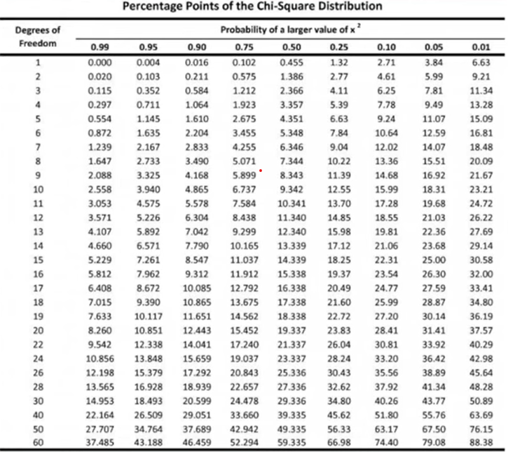
- Use a chi-square table to find the critical value for a chosen significance level (\alpha).
For those curious, the p-value for a chi-square statistic (x) with (k) degrees of freedom is given by the upper-tail integral:
\[p = \int_{x}^{\infty} \frac{1}{2^{k/2}\,\Gamma\!\left(\frac{k}{2}\right)} t^{\frac{k}{2}-1} e^{-t/2} \, dt.\](In practice, we do not compute this integral by hand; we use tables or software.)
Example of Decision
Suppose:
- (\text{df} = 2),
- Significance level (\alpha = 0.05),
- The chi-square table gives a critical value of 5.99.
If our computed (\chi^2 = 6.8) is greater than 5.99, then:
- (\chi^2 > \chi^2_{\text{critical}})
- We reject the null hypothesis.
This means the observed pattern is unlikely to be due to chance alone, under the assumption of independence.
Chi-square Goodness-of-Fit Test (Poisson)
Monthly Guillain–Barré Syndrome Cases in Finland
1. Problem
The table below (Rosner, Chapter 4, with March 1985 excluded) shows the monthly number of Guillain–Barré syndrome cases in Finland from April 1984 to October 1985.
Use the chi-square goodness-of-fit test to assess whether a Poisson distribution is an adequate model for these data.
State your conclusion.
| Month (Year) | # Cases | Month (Year) | # Cases | Month (Year) | # Cases |
|---|---|---|---|---|---|
| April 1984 | 3 | October 1984 | 2 | April 1985 | 7 |
| May 1984 | 7 | November 1984 | 2 | May 1985 | 2 |
| June 1984 | 0 | December 1984 | 3 | June 1985 | 2 |
| July 1984 | 3 | January 1985 | 3 | July 1985 | 6 |
| August 1984 | 4 | February 1985 | 8 | August 1985 | 2 |
| September 1984 | 4 | — | — | September 1985 | 2 |
| Total months | 18 |
Goal
Test whether the monthly case counts follow a Poisson distribution with some mean lambda.
2. Step 1 – Hypotheses
-
Null hypothesis H0:
The monthly count of Guillain–Barré syndrome cases,X, follows a Poisson distribution with meanlambda:X ~ Poisson(lambda) -
Alternative hypothesis HA:
The distribution of the counts is not Poisson.
3. Step 2 – Estimate lambda (mean)
We first estimate the Poisson mean lambda using the total number of cases and the number of months.
Sum of all monthly counts:
3 + 7 + 0 + 3 + 4 + 4 + 2 + 2 + 3 + 3 + 8 + 7 + 2 + 2 + 6 + 2 + 2 + 6 = 66
- Number of months:
n = 18 - Estimated Poisson mean:
lambda_hat = (total number of cases) / (number of months)
           = 66 / 18
           ≈ 3.67
4. Step 3 – Observed Counts by Category
Now count how many months fall into each case value:
- 0 cases: 1 month
- 1 case: 0 months
- 2 cases: 6 months
- 3 cases: 4 months
- 4 cases: 2 months
- 5 cases: 0 months
- 6 cases: 2 months
- 7 cases: 2 months
- 8 cases: 1 month
For the chi-square goodness-of-fit test, we should avoid categories with very small expected counts, so we group values into four categories:
- 0–2 cases
- 3 cases
- 4 cases
- 5 or more cases (5, 6, 7, 8, …)
The observed counts Oᵢ in each category are:
- 0–2:
1 + 0 + 6 = 7 - 3:
4 - 4:
2 - 5 or more:
0 + 2 + 2 + 1 = 5
Summary:
| Category (cases) | Observed count Oᵢ |
|---|---|
| 0–2 | 7 |
| 3 | 4 |
| 4 | 2 |
| ≥5 | 5 |
5. Step 4 – Expected Counts under Poisson
Assume a Poisson distribution with mean lambda_hat = 3.67.
We compute the probability of each category and then convert these to expected counts Eᵢ.
5.1 Poisson probabilities
The Poisson probability mass function (PMF) is:
P(X = k) = e^(-lambda) * lambda^k / k!
Using lambda = 3.67, the needed probabilities (approximate) are:
P(0) ≈ 0.0255
P(1) ≈ 0.0935
P(2) ≈ 0.1716
P(3) ≈ 0.2099
P(4) ≈ 0.1926
Now compute category probabilities.
-
0–2 cases
P(0 ≤ X ≤ 2) = P(0) + P(1) + P(2) ≈ 0.0255 + 0.0935 + 0.1716 ≈ 0.2905 -
3 cases
P(X = 3) ≈ 0.2099 -
4 cases
P(X = 4) ≈ 0.1926 -
5 or more cases
First compute the cumulative probability from 0 to 4:
P(0 ≤ X ≤ 4) ≈ 0.0255 + 0.0935 + 0.1716 + 0.2099 + 0.1926
            ≈ 0.6930
Then
P(X ≥ 5) = 1 − P(0 ≤ X ≤ 4)
         ≈ 1 − 0.6930
         ≈ 0.3070
5.2 Expected counts
For each category, the expected count is
Eᵢ = n * P(category i), n = 18
So:
E_0-2 = 18 * 0.2905 ≈ 5.23
E_3   = 18 * 0.2099 ≈ 3.78
E_4   = 18 * 0.1926 ≈ 3.47
E_≥5  = 18 * 0.3070 ≈ 5.53
Summary:
| Category (cases) | Observed Oᵢ | Expected Eᵢ (Poisson, lambda = 3.67) |
|---|---|---|
| 0–2 | 7 | 5.23 |
| 3 | 4 | 3.78 |
| 4 | 2 | 3.47 |
| ≥5 | 5 | 5.53 |
All expected counts are around 5 or greater, so the chi-square approximation is reasonable.
6. Step 5 – Chi-square Test Statistic
The chi-square goodness-of-fit statistic is:
chi_square = Σ (Oᵢ − Eᵢ)² / Eᵢ
where k = 4 is the number of categories.
Compute each term:
0–2: (7 − 5.23)² / 5.23 ≈ 0.59
3:   (4 − 3.78)² / 3.78 ≈ 0.01
4:   (2 − 3.47)² / 3.47 ≈ 0.62
≥5:  (5 − 5.53)² / 5.53 ≈ 0.05
Then
chi_square ≈ 0.59 + 0.01 + 0.62 + 0.05
           ≈ 1.28
7. Step 6 – Degrees of Freedom and p-value
The degrees of freedom (df) for a chi-square goodness-of-fit test with estimated parameters are:
df = (number of categories) − 1 − (number of estimated parameters)
   = 4 − 1 − 1
   = 2
Summary:
df = 2chi_square ≈ 1.28
From the chi-square distribution with 2 degrees of freedom:
- The p-value is approximately 0.53 (much larger than 0.05).
- The 95% critical value is about
chi_square(0.95, df=2) ≈ 5.99.
Since
1.28 < 5.99
we do not reject the null hypothesis.
8. Step 7 – Conclusion
At the 0.05 significance level:
- We fail to reject the hypothesis that the monthly counts of Guillain–Barré syndrome cases follow a Poisson distribution.
In words:
There is no statistical evidence that the Poisson model is inappropriate for these data.
The Poisson distribution appears to be an adequate model for the monthly case counts.
What to Remember
-
A chi-square test measures how far the observed data deviate from the expected counts under the null hypothesis.
- Use chi-square tests for categorical data:
- Goodness-of-fit: does the data follow a specified distribution?
- Independence: are two categorical variables independent?
- For continuous data (e.g., height, weight), we usually use other tests such as t-tests or ANOVA instead of chi-square.
Reference (Korean video):
https://www.youtube.com/watch?v=lmNZr1EDyNA&t=60s