Null Hypothesis

The null hypothesis is a formal statement (hypothesis) about a population parameter that we treat as the default assumption.

In hypothesis testing, we:

Start by assuming the null hypothesis is true,
Use sample data to see whether there is enough evidence to reject it.

T-test

The t-test is one of the main methods used to test a null hypothesis about means.

It can be used even when the sample size is larger than 30; that is not a problem.
When the sample size is large, results from the t-test and z-test are very similar.

The key point is not just the sample size, but whether we know the population variance:

When the sample size is small and the population variance is unknown, the t-test is especially useful.
This is because the t-test is based on the t-distribution.

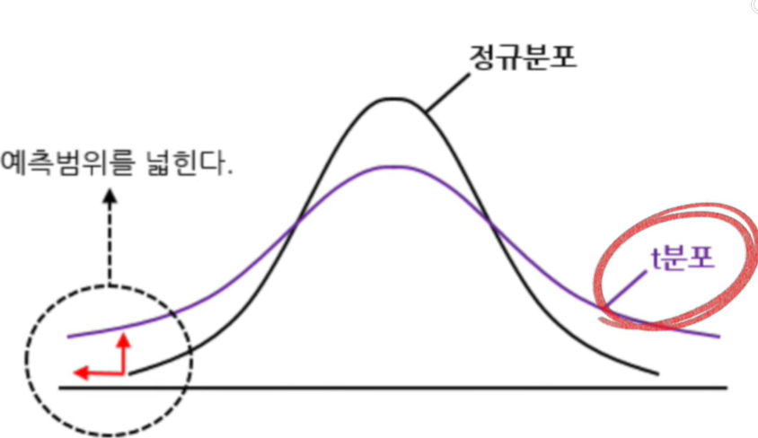
Why t-distribution?

The normal distribution has a high peak near the mean and thin tails.
The t-distribution has a lower peak near the mean and heavier tails, which better reflects the chance of more extreme values.

Because the t-distribution has heavier tails, it captures the extra uncertainty that arises when:

We have a small sample, and
We must estimate the standard deviation from the sample itself.

So, in situations with small (n) and unknown variance, the t-test is more appropriate than a z-test.

t-vs-normal

Example Scenario

We want to compare which class is better at math: Class A or Class B.

Class A: sample size 12, mean 80, standard deviation 5.
Class B: sample size 10, mean 85, standard deviation 6.

Just looking at the means, Class B appears better. But:

Is this difference statistically significant, or could it be due to random sampling?

For example, if the sample from Class A happens to include mostly weaker students by chance, the observed difference might be misleading.

The t-test evaluates:

How large the difference in means is
Relative to the variability (noise) in the data.

In other words, the t-test measures whether the gap between means is likely to be just random fluctuation.

Types of T-tests

One-sample t-test
- Compares a sample mean to a specific value (e.g., national average).
- Example: test whether a school’s average math score is different from the national average.
Independent two-sample t-test
- Compares means of two independent groups.
- Example: test whether the mean exam scores of Class A and Class B differ significantly.
Paired t-test (dependent samples)
- Compares two measurements on the same group (or matched pairs).
- Example: compare students’ scores before vs. after applying a new teaching method.

Setting Up the T-test

To show that the higher mean of Class B is not just due to chance, we set:

Null hypothesis (H_0):
The mean scores of Class A and Class B are equal (no difference).
Alternative hypothesis (H_1):
The mean scores of Class A and Class B are different.

As with z-tests:

If the p-value is less than the chosen significance level (\alpha), we reject the null hypothesis.

In terms of the t-test:

If the absolute t-value is greater than the critical value from the t-table, we reject (H_0).

Two-sample t Statistic (Equal Variance Assumption)

For two groups (assuming equal variances), the t statistic is

\[t = \frac{\overline{X}_{1}-\overline{X}_{2}} {\sqrt{\,s_p^{2}\!\left(\frac{1}{n_{1}}+\frac{1}{n_{2}}\right)}}\]

where the pooled (common) sample variance is

\[s_p^{2} = \frac{(n_{1}-1)s_{1}^{2} + (n_{2}-1)s_{2}^{2}}{\,n_{1}+n_{2}-2\,}.\]

Plugging in the Numbers

For Class A and Class B:

Class A: (n_1 = 12), mean = 80, (s_1 = 5).
Class B: (n_2 = 10), mean = 85, (s_2 = 6).

Compute the pooled variance:

\[\begin{aligned} s_p^{2} &= \frac{(12 - 1)(5^{2}) + (10 - 1)(6^{2})}{12 + 10 - 2} \\ &= \frac{11 \cdot 25 + 9 \cdot 36}{20} \\ &= \frac{275 + 324}{20} = \frac{599}{20} = 29.95. \end{aligned}\]

Therefore,

\[s_p = \sqrt{29.95} \approx 5.47.\]

Now compute the t-value:

\[\begin{aligned} t &= \frac{80 - 85}{\sqrt{\,29.95\!\left(\frac{1}{12}+\frac{1}{10}\right)}} \\ &= \frac{-5}{\sqrt{\,29.95 \times 0.183\overline{3}\,}} \\ &= \frac{-5}{2.34} \approx -2.13. \end{aligned}\]

Drawing the Conclusion

Degrees of freedom and significance level:

\[\text{df} = n_1 + n_2 - 2 = 20,\] \[\alpha = 0.05.\]

For a two-sided test with (\alpha = 0.05) and (\text{df} = 20), the critical t-value is approximately:

(t_{\text{crit}} \approx \pm 2.086).

We compare the absolute t-value:

( t = 2.13 > 2.086 = t_{\text{crit}} ).

Since the t-value lies outside the acceptance region, we reject the null hypothesis at the 5% significance level.

Interpretation:
The difference in mean scores between Class A and Class B is statistically significant at (\alpha = 0.05); it is unlikely to be due to chance alone.

PREVIOUSEstimation

NEXTANOVA