1. What is Regression Analysis?
Regression analysis is
A method to mathematically model causal relationships,
asking which variables act as causes for another variable.
- Variables that act as causes: independent variables (explanatory variables)
- Variable that is affected as a result: dependent variable (response variable)
Example notation:
x1, x2, x3, x4  →  y
(independent vars)   (dependent var)
2. Basic Types of Regression
- By number of independent variables
- 1 independent variable: simple regression
- 2 or more independent variables: multiple regression
- By the scale/type of independent and dependent variables
- Various regression models exist depending on whether variables are continuous or categorical.
- By relationship shape
- Linear regression: relationship is expressed as a straight line
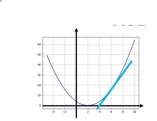
y = a x + b - Nonlinear regression: relationship is expressed as a curve
e.g.,y = a x² + b,y = exp(a x), etc.
- Linear regression: relationship is expressed as a straight line
3. Intuitive Meaning of Linear Regression
Linear regression assumes:
The relationship between two variables can be approximated by a straight line,
and among all possible lines, we find the one that best explains the data.
So the goal of linear regression is:
"Find the line that best represents the data points."
4. Car Example (Speed → Braking Distance)
A simple intuitive example:
- A car is moving and the driver hits the brake.
- Speed at the moment of braking:
x(km/h) - Distance traveled until a complete stop:
y(m)
Intuitively we know:
The higher the speed x, the longer the braking distance y.
We use regression analysis to express this relationship mathematically.
- Perform many experiments and collect
(x, y)data pairs (e.g., 50 trials). - Draw a scatter plot: we see an overall upward trend.
- We then find a single line that “best passes through” these points → linear regression.
| x | y | \hat{y} | error |
|---|---|---|---|
| 1 | 3 | 0.5 | 2.5 |
| 2 | 5 | 1 | 4 |
Cost function:
\[C(m,b) = \frac{1}{2}\Big( y_1 - (m x_1 + b) \Big)^2 + \frac{1}{2}\Big( y_2 - (m x_2 + b) \Big)^2\]Partial derivative with respect to (m):
\[\frac{\partial C}{\partial m} = \frac{\partial}{\partial m} \left[ \frac{1}{2}\Big( y_1 - (m x_1 + b) \Big)^2 + \frac{1}{2}\Big( y_2 - (m x_2 + b) \Big)^2 \right]\]Using the chain rule step-by-step:
\[\frac{\partial C}{\partial m} = \frac{1}{2} \cdot 2\Big( y_1 - (m x_1 + b) \Big)\frac{\partial}{\partial m}\Big( y_1 - (m x_1 + b) \Big) + \frac{1}{2} \cdot 2\Big( y_2 - (m x_2 + b) \Big)\frac{\partial}{\partial m}\Big( y_2 - (m x_2 + b) \Big)\]Since (\dfrac{\partial}{\partial m}(y_i - (m x_i + b)) = -x_i),
\[\frac{\partial C}{\partial m} = -\Big( y_1 - (m x_1 + b) \Big)x_1 -\Big( y_2 - (m x_2 + b) \Big)x_2\]Gradient w.r.t. m (example with two points)
\[\frac{\partial C}{\partial m} = \frac{1}{2} \Big( 2 \big( y_1 - (m x_1 + b) \big)(-x_1) + 2 \big( y_2 - (m x_2 + b) \big)(-x_2) \Big)\]Using (\hat{y}_i = m x_i + b):
\[\frac{\partial C}{\partial m} = \frac{1}{2} \Big( 2 (y_1 - \hat{y}_1)(-x_1) + 2 (y_2 - \hat{y}_2)(-x_2) \Big)\]Let (\text{error}_i = y_i - \hat{y}_i):
\[\frac{\partial C}{\partial m} = \frac{1}{2} \Big( 2 \,\text{error}_1\,(-x_1) + 2 \,\text{error}_2\,(-x_2) \Big)\]For the specific numbers
((x_1 = 1, x_2 = 2, \text{error}_1 = 2.5, \text{error}_2 = 4)):
Gradient w.r.t. b and update step
From the same cost function,
\[\frac{\partial C}{\partial b} = \frac{1}{2} \Big( 2 (y_1 - (m x_1 + b))(-1) + 2 (y_2 - (m x_2 + b))(-1) \Big)\]Using (\hat{y}_i = m x_i + b) and (\text{error}_i = y_i - \hat{y}_i):
\[\frac{\partial C}{\partial b} = -\text{error}_1 - \text{error}_2\]For (\text{error}_1 = 2.5, \text{error}_2 = 4):
\[\frac{\partial C}{\partial b} = -(2.5 + 4) = -6.5\]Gradient descent update:
\[b_{\text{new}} = b_{\text{old}} - \alpha \frac{\partial C}{\partial b}\]With (b_{\text{old}} = 0) and (\alpha = 0.01):
\[b_{\text{new}} = 0 - 0.01 \cdot (-6.5) = 0 + 0.065 = 0.065\]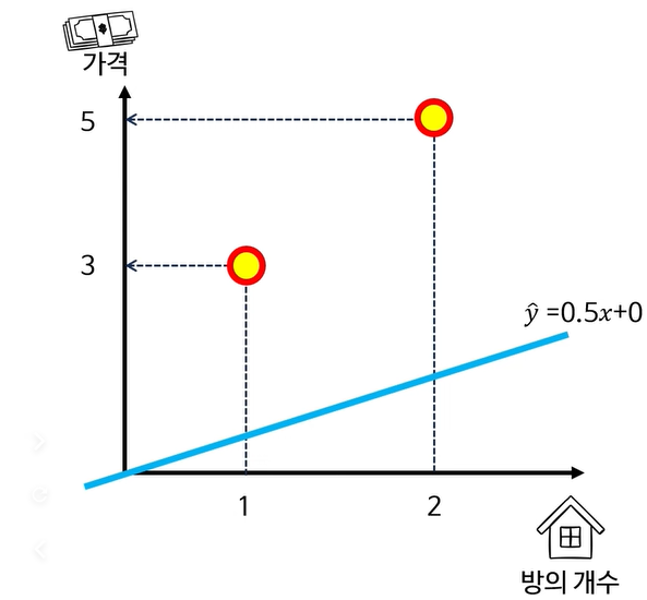
5. Concept of Residuals
When we draw one straight line, the data points will not lie exactly on the line.
- A data point:
(xᵢ, yᵢ) - Predicted value on the regression line:
ŷᵢ = a xᵢ + b
The residual is:
residual = actual value yᵢ − predicted value ŷᵢ
On the graph:
- It is the vertical distance between the point
(xᵢ, yᵢ)and the point(xᵢ, ŷᵢ)on the line.
The smaller the residual,
the better the line explains that point.
6. Idea of the Least Squares Method
Question:
“Which line best explains the data?”
→ We need a criterion.
6.1 Minimizing the Sum of Squared Residuals
For each point, we compute the residual and then consider the sum of their squares:
residualᵢ = yᵢ − ŷᵢ
Sum of squared residuals S = Σ (residualᵢ)²
The goal of the least squares method is:
Choose a, b such that
S = Σ (yᵢ − ŷᵢ)² is minimized.
- Why square the residuals?
- To remove the sign (±)
- To make it easier to find the minimum using calculus (partial derivatives)
- The line obtained this way is called the least squares regression line.
7. Advantages of the Least Squares Regression Line
- Quantitative description of causal relationships
- Instead of just saying “they are related,”
we express a numeric relationship viay = a x + b.
- Instead of just saying “they are related,”
- Prediction for new data
- Example: if a newly measured speed is
x = 23 km/h,
we can plug it into the regression equation to predicty, the braking distance. - It won’t be perfectly accurate, but
it provides a reasonable estimate.
- Example: if a newly measured speed is
8. How Do We Actually Find the Line? (Briefly)
The video mentions two mathematical approaches:
- Using partial derivatives
- Treat the sum of squared residuals
S(a, b)as a function ofaandb. - Take partial derivatives and solve:
∂S/∂a = 0,∂S/∂b = 0.
- Treat the sum of squared residuals
- Using matrices (linear algebra)
- Represent all data points in matrix form.
- Find the least squares solution using the normal equations or other linear algebra tools.
For basic understanding, it is enough to know:
“We find the coefficients a, b using mathematical tools so that the sum of squared residuals is minimized.”
9. One-Sentence Summary
- Regression analysis: a tool to mathematically model how independent variables affect a dependent variable.
- Linear regression:
assumes a linear relationship likey = a x + b,
and finds the line that minimizes the sum of squared residuals (least squares). - With the resulting regression equation, we can:
- interpret causal relationships quantitatively, and
- predict new outcomes.
10. Why Is “Linear” So Confusing?
When students first see regression, they usually see examples like:
x = height,y = weight- The scatter plot looks roughly like a straight upward line
- So we fit a line like
y ≈ a x + b→ linear regression
So many people think:
“Linear regression = analysis used when x and y have a straight-line relationship.”
But this is only half of the story.
The key point of the lecture is that this is an incomplete understanding.
11. What Really Needs to Be Linear?
In linear regression, what truly needs to be linear is:
Not the input x, but the parameters (coefficients).
In other words, the model is called linear if it can be written as:
y_hat = a * (something) + b * (something else) + c * (another thing) + ...
and this expression is a first-degree (linear) function in the parameters a, b, c, etc.
If the parameters are multiplied together or squared, the model becomes nonlinear in the parameters.
Examples:
y = a * x + b- Linear in a and b → linear model
y = a * x^2 + b * x + c- Curved in x, but linear in a, b, c → still linear regression
y = a^2 * xory = a * b * x- Parameters are multiplied or squared → not linear in a, b → nonlinear regression
So:
“Linear regression = regression that is linear in the parameters.”
(The model does not have to be a straight line in x!)
12. Nonlinear Feature Transformations Are Okay
Even if we transform x in a nonlinear way, the model can still be linear.
For example, we can define:
z1 = x
z2 = x^2
z3 = log(x + 1)

y_hat = a * z1 + b * z2 + c * z3 + d
- As a function of x, this may represent a complex curve.
- But the model is linear in a, b, c, d.
- Therefore, this is still linear regression.
So it is more accurate to say that linear regression
models y as a linear combination of transformed features
phi(x)
(i.e., linear in the parameters, not necessarily linear in the raw input x).
13. Why Is “Linear in Parameters” Important?
Being linear in the parameters has several advantages:
- Solvable by least squares in a nice way
- The sum of squared residuals
S(w)becomes a convex function. - We can find the solution analytically or numerically in a stable way using calculus and linear algebra.
- The sum of squared residuals
- Easy to interpret
- Each coefficient a, b, c represents “how much one feature affects y”.
- For example, if
a > 0, increasingz1tends to increase y.
- Directly connected to deep learning
- A neural network layer does:
y = W x + b→ linear in weights W and bias b. - Deep networks stack such linear layers with nonlinear activation functions (ReLU, sigmoid, etc.).
- A neural network layer does:
14. How to Check If a Model Is Linear
You can ask this question:
Q. The input x can go through any complicated transformation.
But is the final expression a first-degree (linear) function of the parameters?
That is, of the form
coef1 * f1(x) + coef2 * f2(x) + ...?
- Yes → linear model (linear regression)
- No → nonlinear model (nonlinear regression)
15. Final Takeaway
In linear regression, the word “linear” does not mean
“x and y have a straight-line relationship”.
It means the model is linear in its parameters (coefficients).
If you keep this viewpoint:
- Polynomial regression, feature transformations,
- and linear layers in deep learning networks
will all look much clearer, and you can always first ask:
“Is this model linear in the parameters?”